
Assortative mating and differences
Understanding through simulations

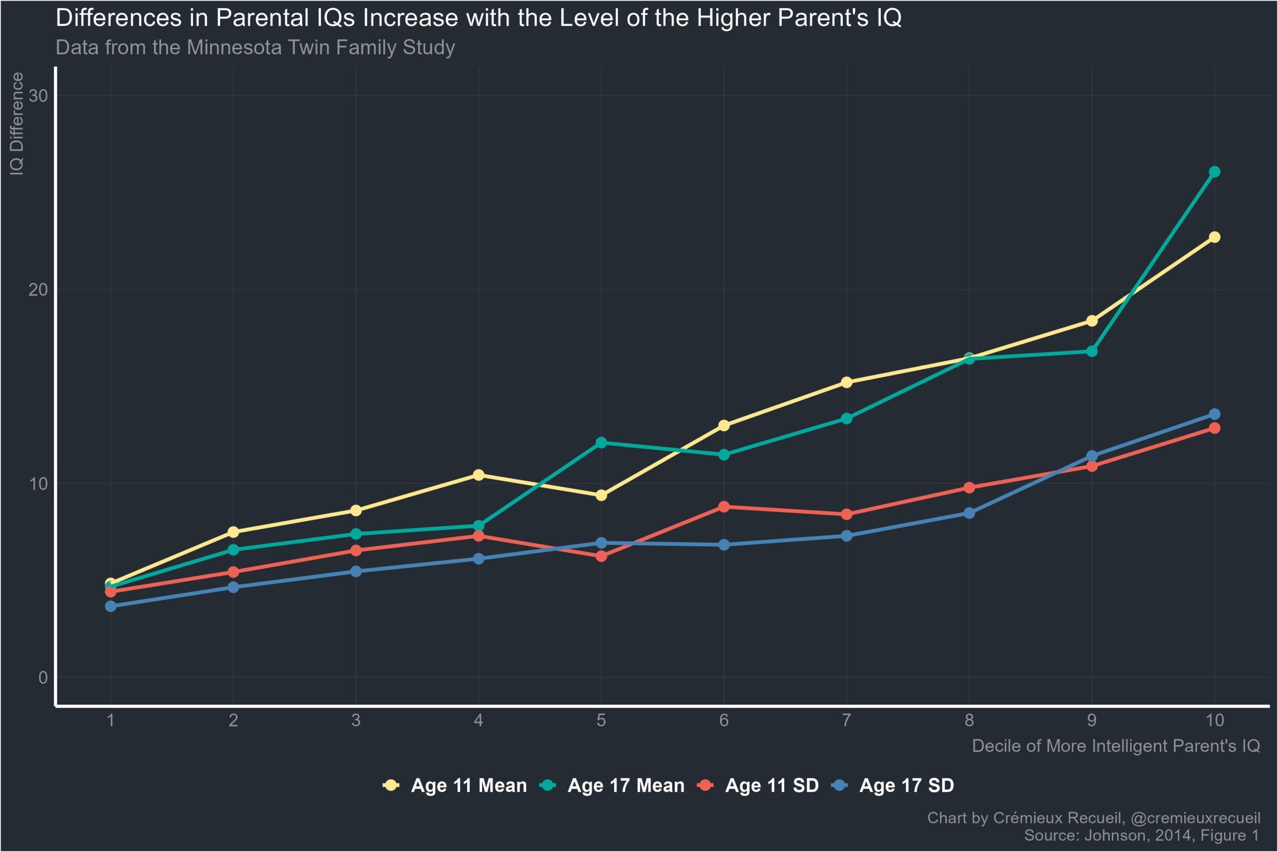
Cremieux has a viral post showing the absolute IQ gaps for spouses/partners as a function of the smartest spouse:
This finding is trivial but apparently surprising to many people judging from the 400+ comments. Assortative mating appears to be nonlinear. This is not true as such, it is linear since it is just a correlation of two variables. So let’s understand how this works. I’ve simulated 50 men and women and paired them up according to different degrees of assortative mating:
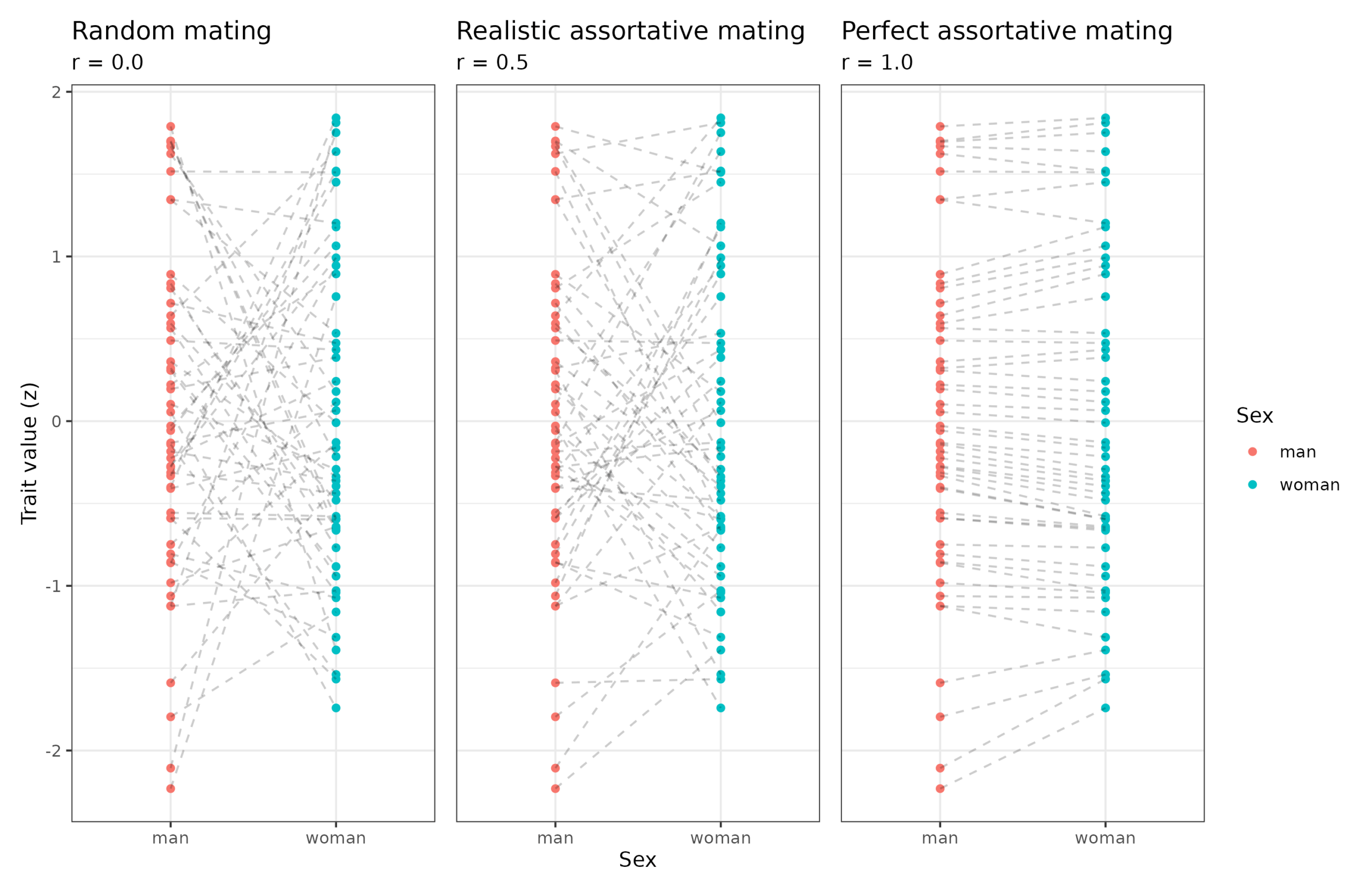
The lines show the pairings. The leftmost plot shows random pairings (r close to 0, in this case -0.06), the middle shows strong assortative mating (as seen for intelligence, politics, religiousness, r close to 0.5, here 0.59) and the rightmost plot shows perfect assortative mating under the constraints of the finite pool of partners (r close to 1, in this case 0.99). The absolute gaps for the pairings are: 1.11, 0.74, and 0.13 SD. Or in IQ terms, 16.7, 11, and 2 IQ points on average. If we sort them by highest score within a pair, we get the same result as in Crem’s real life data:
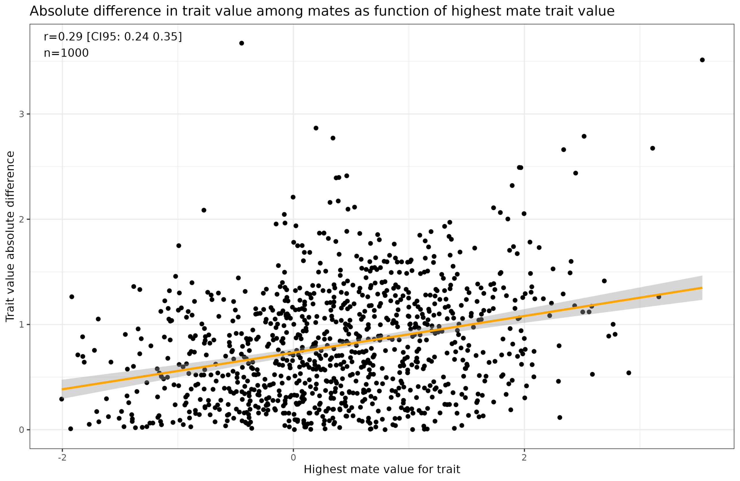
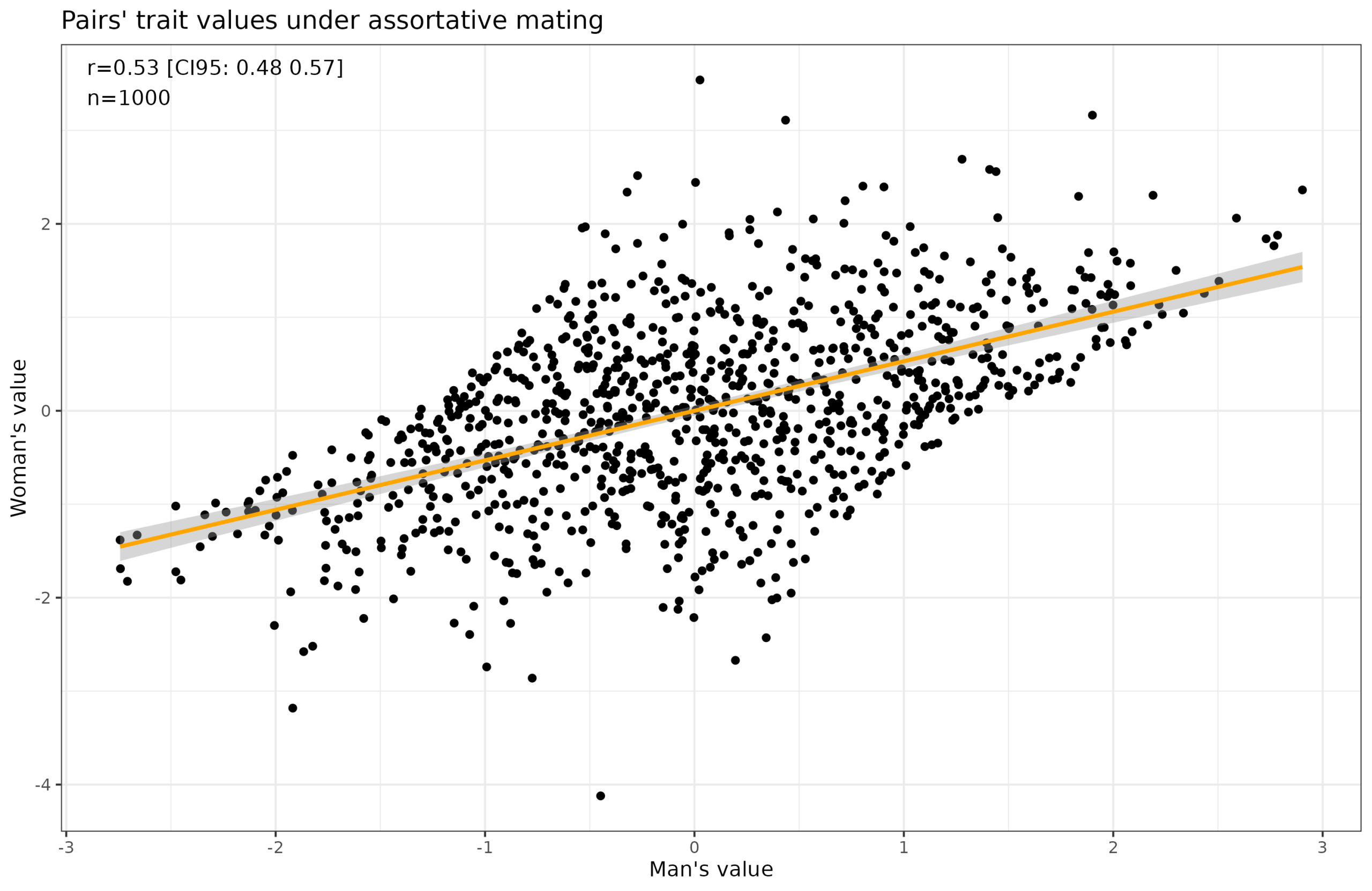
To show this pattern I simulated 1000 pairs instead of 50 since that is too small to reliably show this correlation of about 0.30. Here’s a comparison of the 3 scenarios:
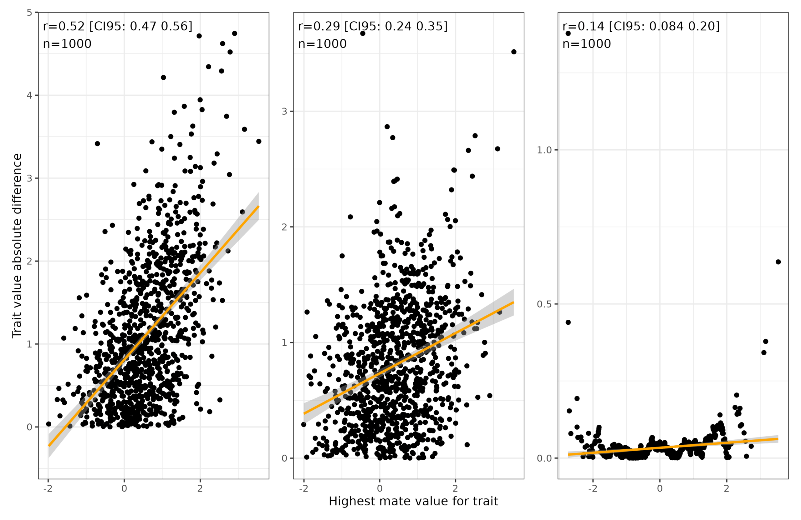
We can clearly see that the correlation diminishes as a function of the assortative mating correlation. This is basically just plotting the regression towards the mean since the spouse of the highest value partner is always closer to the mean.
What’s the mathematics behind this? Assortative mating just means that pairs are correlated for some trait. This relationship is linear:
(The pattern is perhaps a bit goofy looking due to the way I paired up people. Some kind of pairing algorithm is needed, and I used the noise approach.)
The expected value of a woman is just the man’s value times the correlation. Thus, a man with trait value 2 under correlation of 0.5 has on average a woman with a value of 1. This holds in both directions bidirectionally, thus a woman with a value of -2 has on average a man with a value of -1 and so on. Thus in absolute terms, the expected difference is larger the further out on the tail of the distribution a given person is. There is nothing mysterious here, Crem’s plot is in fact a trivial, as he also says:
This is almost tautological, but when you state it, I’ve found that it still surprises some people. Tautology != obvious. Sort the other way and you can get the reverse finding, too, but those pairings are quite uncommon!
Source is Wendy Johnson’s 2014 ISIR presentation.
I think the issue is that people imagine that assortative mating means that people pick spouses within a particular distance from themselves. They do this, but only on average. As we saw above, given a spousal correlation of 0.5, the average gap is 11 IQ points. But it’s a mistake to that this number and reason backwards and be surprised. The expected IQ gap is a function of the average IQ or highest IQ of the couple, not an invariant number. The gaps will be larger for mates with more extreme values.
For reference, here are some typical measured human assortative mating results from Horwits et al 2023:
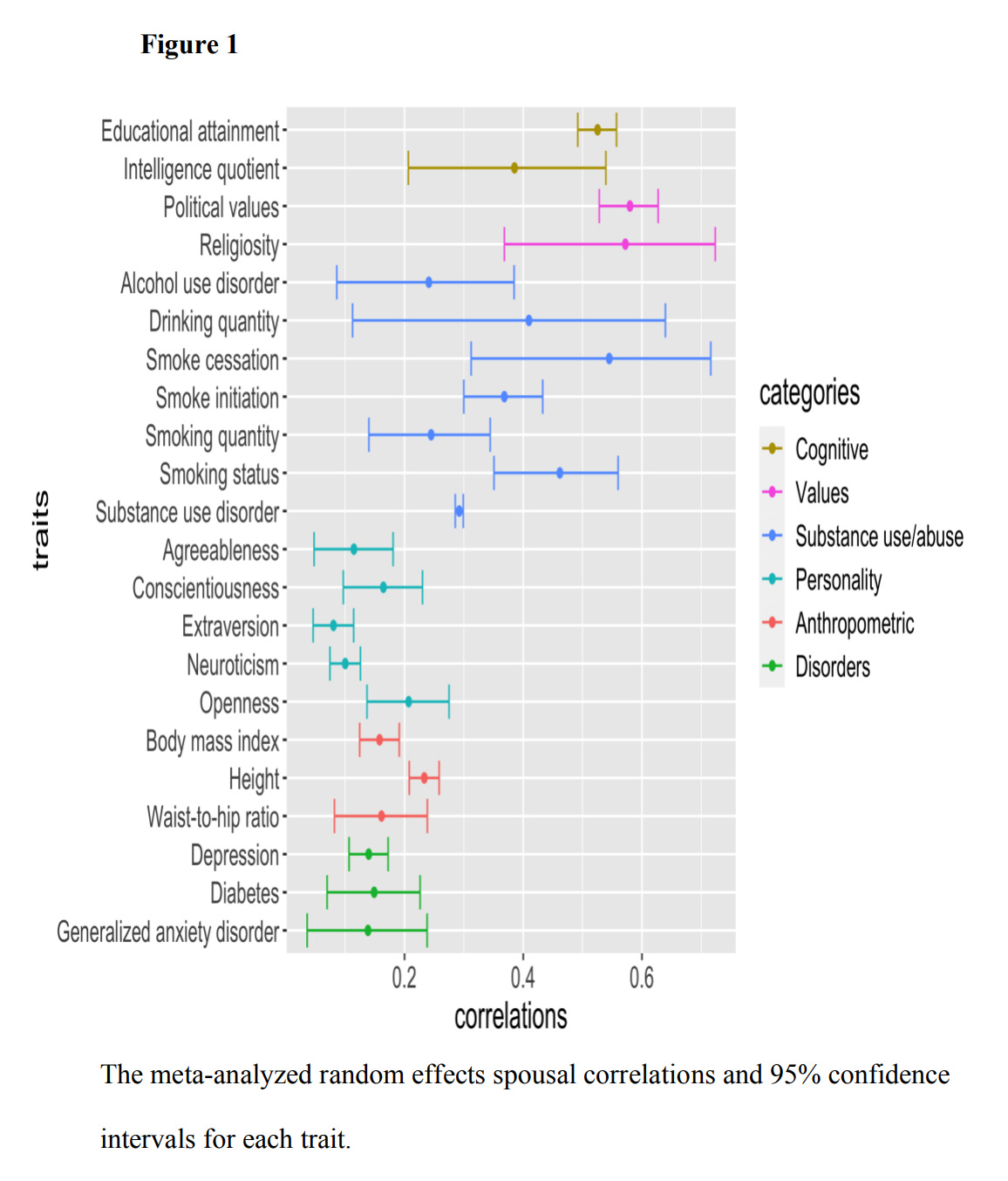
They reported a value for measured IQ of about 0.40, but measurement errors in the variables make them a bit too low. I imagine when adjusted for unreliability, the true correlation will be around 0.50, which is why I used that value above. Not shown here, but the correlation for age is usually around 0.90.
Nice explanation.
One thing I found myself wondering above was how much quantitative deviation the real data has from the idealized model. One could easily imagine social rarity effects impacting the average differences as well, but they might be pretty small relative to uncertainty in the quantificatiom of assortative mating. For example, social sorting is imperfect, in the sense that an extreme person's entire social pool will show regression to the mean, which will limit their ability to fully express their preferences in partner selection. This should make the differences in real data even more extreme than in a global information matching model.
It would be nice to see a social selection theory paper on how selection "power" grows with group size, just like it does for natural selection, come to think of it. The math is probably basically the same, but there might be some interesting twists to the social setting.
https://adamgolding.substack.com/p/sumerian-sperm-competition