Differential measurement error and regression
In reviewing our upcoming target article in Mankind Quarterly (edit: now published), Gerhard Meisenberg wrote:
“One possibility that you don’t seem to discuss is that there are true and large correlations of the Euro% variable and the geographic variables, but that the geographic variables are measured much more precisely than the Euro% variable. In that case, regression models will produce independent effects of the more precisely measured geographic variables even if they have no causal effects at all, because they capture some of the variance that is not captured by the Euro% variable due to its inaccurate measurement”.
I had noticed this problem before and tried to build a simulation to show it. Unfortunately, I ran into problems due to not knowing about mathematical statistics (see here).
Suppose the situation is this:

So, we have a causal network where X1 causes both X2 and Y. We also model the measurement error aspect of each variable.
Now, suppose that we don't know whether X1 or X2 causes Y, and that we plug them into a multiple regression model together with Y as the outcome. If we measured all variables without error, the model would find that X1 predicts Y and that X2 doesn't.
However, suppose that we can measure X2 and Y without error and X1 with some error. What would we find? We would find that X2 seems to predict Y, despite we knowing that it has no causal effect on Y at all.
For instance, we can simulate this situation in R using the following code:
# differential measurement error ------------------------------------------
library(pacman);p_load(magrittr, lavaan, semPlot, kirkegaard)
set.seed(1)
n = 1000
{
  X1 = rnorm(n)
  X1_orb = (X1 + rnorm(n) * .6) %>% scale() #lots of measurement error
  X2 = (X1 + rnorm(n)) %>% scale()
  X2_orb = X2 #no measurement error
  Y = (X1 + rnorm(n)) %>% scale()
  Y_orb = Y #no measurement error
  d = data.frame(X1, X1_orb, X2, X2_orb, Y, Y_orb)
}
#fit
#true scores
lm("Y ~ X1 + X2", data = d) %>% lm_CI()
#observed scores
lm("Y_orb ~ X1_orb + X2_orb", data = d) %>% lm_CI()
What do the results look like?
$coefs
   Beta   SE CI.lower CI.upper
X1 0.68 0.03     0.62     0.74
X2 0.01 0.03    -0.05     0.07
$effect_size
       R2   R2 adj.
0.5100199 0.5090370
$coefs
Beta SE CI.lower CI.upper
X1_orb 0.48 0.03 0.42 0.54
X2_orb 0.22 0.03 0.16 0.28
$effect_size
R2 R2 adj.
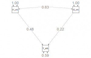
0.4112067 0.4100255Thus, we see that in the first case, multiple regression found X2 to be a useless predictor (beta = .01); in the second case, it found X2 to be a useful predictor with a beta of .22. In both cases X1 was a useful predictor, but it was weaker in the second case (as expected due to the worse measurement).
Multiple regression can also be visualized using path models. So let's try that for the same models as above. R:
#path models
#1
model = "Y ~ X1 + X2"
fit = sem(model, data = d)
semPaths(fit, whatLabels = "std")
#2
model = "Y_orb ~ X1_orb + X2_orb"
fit = sem(model, data = d)
semPaths(fit, whatLabels = "std", nCharNodes = 0)
The plots:

Thus, we see that these show about the same numbers as multiple regression. I think the difference is due to them using different methods of fitting the numbers (sem() uses maximum likelihood by default). So, we have a general problem for our modeling: when our measures have measurement error, this can impact our findings and not just in the way of finding smaller numbers as with zero-order correlations.
One could set up some causal networks and try all the combinations of measurement error in variables to see how it affects results in general. From the above, I would guess that it tends to make simple systems seem more complicated by spreading out the predictive ability across more variables that are correlated with the true causal variables (false positives).

