
What did the new WGS UKBB study show?
A nice improvement, the next path forward and reliability issues

I wasn’t going to blog this, since I prefer not covering the same ground as others, but due to multiple requests and questions, I will cover it anyway. It’s this new study from the Yengo group:
Wainschtein et al 2025. Estimation and mapping of the missing heritability of human phenotypes.
Rare coding variants shape inter-individual differences in human phenotypes1. However, the contribution of rare non-coding variants to those differences remains poorly characterized. Here we analyse whole-genome sequence (WGS) data from 347,630 individuals with European ancestry in the UK Biobank2,3 to quantify the relative contribution of 40 million single-nucleotide and short indel variants (with a minor allele frequency (MAF) larger than 0.01%) to the heritability of 34 complex traits and diseases. On average across phenotypes, we find that WGS captures approximately 88% of the pedigree-based narrow sense heritability: that is, 20% from rare variants (MAF < 1%) and 68% from common variants (MAF ≥ 1%). We show that coding and non-coding genetic variants account for 21% and 79% of the rare-variant WGS-based heritability, respectively. We identified 15 traits with no significant difference between WGS-based and pedigree-based heritability estimates, suggesting their heritability is fully accounted for by WGS data. Finally, we performed genome-wide association analyses of all 34 phenotypes and, overall, identified 11,243 common-variant associations and 886 rare-variant associations. Altogether, our study provides high-precision estimates of rare-variant heritability, explains the heritability of many phenotypes and demonstrates for lipid traits that more than 25% of rare-variant heritability can be mapped to specific loci using fewer than 500,000 fully sequenced genomes.
It is the much awaited study using GREML-like methods to estimate heritability in the large UKBB cohort. Recall that GREML-like methods use distant relatives who happen to share a slight genetic overlap somewhere to estimate heritabilities. Essentially, regress similarity (or dissimilarity) in some phenotype on all pairwise distant genetic overlaps in a sample. Most people are not detectably related, but some people have e.g. 1% genetic overlap, some have 2% etc. These are 2+ cousins and the like. The people who have 2% overlap will be very slightly more similar than those with 1% overlap. If one has enough data, one can estimate this slope and extrapolate it to 100% overlap (same egg twins), and the predicted average difference. If this is e.g. 2 cm in height, one can convert this to a correlation metric which is then the heritability (the real value is about 2cm or r = .90 or so). The details are more complex, but this is the simplified version.
This kind of method has been used for years, first from the original GCTA software (GREML is the method) and then later software tools. Though many studies talk about heritability, they are in fact usually not estimating the same value (estimand). For instance, the predictive validity of a polygenic score tells us how much we can currently predict a given phenotype using measured genetic variants and some genetic prediction model (’GWAS’) we have trained. The square of this value is the PGS heritability. Now, our models are not perfect in part because they are not trained with an infinitely large sample size. GREML-like methods (in theory) tell us how good a model would be if it had infinite sample size. This is usually called the SNP heritability because it is based on SNP genetic variants (single letter variations). This is not the full genetic effect because many genetic variations are single letter variations, but it is a lower bound value. Family or pedigree studies use relationships among relatives to partition the variance into unobserved causes (variance components), which include genetics and various kinds of non-genetic causes. Depending on the specific design, the value estimated here may be additive heritability or broad (full) heritability. The difference is that the additive heritability only includes genetic effects that “add up”. That is to say, it includes genetic variations where having 2 copies of some variant gives twice the effect of 1 copy. Thus, if in some position having “T” as opposed to “G” results in being 0.5 cm taller, then if additivity rules (it mostly does), then having 2 copies yields 2*0.5=1cm. Broad heritability includes any remaining more complex effects which means effects of genetic variants that depend on other genetic variants for their effects, or which are nonlinear. That is, maybe having 2 “T”’s makes you -1cm shorter not +cm taller (all of this is called dominance). Genetic effects that depend on others might mean that having “T”’s at some position makes you 0.5cm taller only if you have “A” at some other position and otherwise does nothing (epistasis).
Anyway, so the next time you wonder why results provide seemingly inconsistent results it is because they aren’t estimating the same value (estimand) in general. Nevertheless, there is a somewhat unhelpful term about these differences, called the missing heritability. It sounds ominous but it just means, for instance, that though we have trained a genetic model to predict some phenotype, and it does OK, say it predicts with r = 0.30, our GREML study tells us that if we just had an infinite number of people to fit the model on (and an infinite powerful computer to do this with or infinite time to wait), then the model would predict at r = 0.60. In this case, the heritability values would be 0.30²=9% and 0.60²=36%, so the missing heritability is 27%. You can see how this is misleading because the difference in validity is a factor of 2, not 4. Variances are deceptive.
Anyway, since almost all prior using estimating GREML-like (SNP) heritability used data from arrays, there was another problem. Arrays don’t measure the whole genome, they just measure (mostly) SNPs distributed around the genome, usually 600k to 200k of them. Based on these measured variants, one can fill in (impute) best guesses for the unseen variants, yielding typically about 10M variants. These are then fed into the various models. This data quality leads to some decreases in the model fit since it is being given partially uncertain data and thus the number produced will be an underestimate even of the estimand desired. This is another of the reasons the GREML-like results are always smaller than family based models. There are further issues, such as the exclusion of variants too rare to estimate properly, which further bias the values downwards (if rare variants are important). The solution to most of these problems is to use actual whole genome data (deep whole genome sequencing), which is more expensive but has been falling in price dramatically for decades. Their new results in a figure:
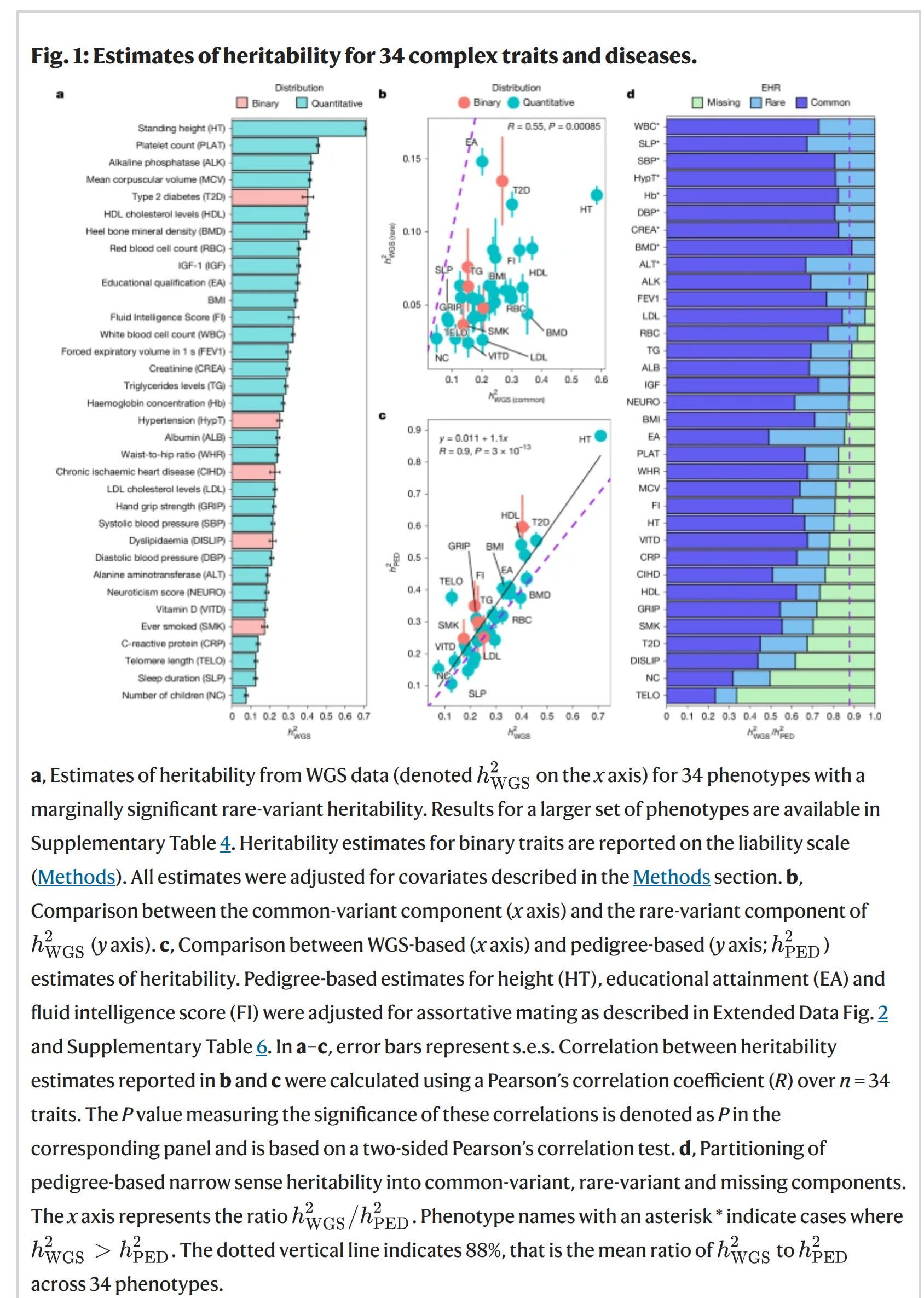
The left plot shows their heritability estimates from the WGS data using GREML. It looks like height showed a heritability of 71%. This is still not the same as the family data, which for clinically measured height usually reaches 90%. 90% means that a perfect model capturing this would predict with r = 0.95. What has gotten many people talking is that the fluid intelligence score showed a value of 33% and educational attainment one of 35%:

Actually, since this fluid intelligence test is just 13 items and has a reliability of 0.61 (among a sample who it twice). As such, the value should be corrected for the reliability issue, which (since it is a variance) is just dividing by the reliability is 55%. This is still lower than the usual 80-85% values from family studies (in adults). The difference comes from deficiencies in the modeling (not all variants are included, only additive effects), and probably likely also because a single test cannot measure general intelligence entirely correctly (the g-loading is below 1). Nevertheless, it sets a new minimum value that Gusev et al can have fun explaining away.
The right-side plot compares their family estimates to their GREML WGS estimates to quantify any missing heritability in the sense defined above. The big claim here is that a lot of the missing heritability has been removed from the usage of WGS data as hereditarians had expected. However, it is odd that their family estimates are somewhat low for some traits. Fluid intelligence was 41%, BMI 39%, but height was a normal 88%. Fluid intelligence corrected for unreliability is 67% which is not so far from the usual values. Unfortunately, the authors aren’t very clear on the exact pedigree (family) model used. They just say:
Pedigree-based estimates of narrow sense heritability were obtained from a set of 171,446 pairs of relatives (GRM value greater than 0.05) identified in the UKB.
Which family members? Doesn’t say anywhere, and I skimmed the various supplements too. Odd.
They additionally did some new GWASs using the new and improved dataset, but since the sample size is much smaller than existing GWASs, this is not fantastically useful, and they mostly didn’t find rare variants of interest (except for lipids).
Anyway, I hope this provides a useful summary for those who sent questions. It is a nice step forward to be sure, and the next step should be to add the non-SNP variants. Actually estimating them is tough even with deep WGS data because they are usually longer than the small stretches of DNA that UKBB’s WGS used, which I think is 2x150 (read strings of 150 basepairs forwards and backwards, or each strand). Any variant that is longer than 150 letters is thus hard to map correctly. Anyway, some of these longer variants (called structural variants, or SVs) can be estimated and included in genetic models. This should provide a small increase in validity. To properly measure them, they need to upgrade the data again to long-reads WGS. This is probably many years away from now unless prices fall even faster.
Very helpful. Thanks for providing.
> Nevertheless, it sets a new minimum value that Gusev et al can have fun explaining away.
I was also quite curious how Sasha would respond to this. The answer is in a comment, and it is overall a good answer IMO (apart from the 1-dimensional claim)—& I have developed a similar method as the Spearman correction that further generalizes to other scenarios: https://theinfinitesimal.substack.com/p/the-missing-heritability-question/comment/180857849.
For me, at least, I’ll default to Sasha’s explanation until this particular question has a more direct study to measure it