Whose benefit of the doubt?

Costs related to imperfect decision making must be borne by someone

In selection contexts (e.g. hiring), there is the notion of the benefit of the doubt. If you have some non-meritocratic desires for selection, and you find yourself with 2 otherwise (almost) equal candidates, you can choose to give the benefit of the doubt to the one who you prefer for non-meritocratic reasons. It could be your friend, a family member, or a member of whatever population subgroup you like. Whatever the reason, that person ends up selected and the other one de-selected. Normally, we think about this in the context of the benefits to the selected person if they are members of some ‘protected group’ in some legal context (e.g. lower castes in India). However, here I want to broaden the topic to include the full game theory approach of costs and benefits.

First, let’s consider the basics of the scenario. Here we consider two groups, the blues and the greens, of which there are 10,000 candidates each. Some of them are being picked for some purpose which results in them getting some benefit. Whoever is doing the selection is picking the top 10% of candidates (2000 persons). The groups differ in some underlying trait by 1 SD, which has been measured with an imperfect assessment (reliability = 0.75, that is, correlation with true value of 0.87). Furthermore, some statisticians have tried various adjustments to the scores:

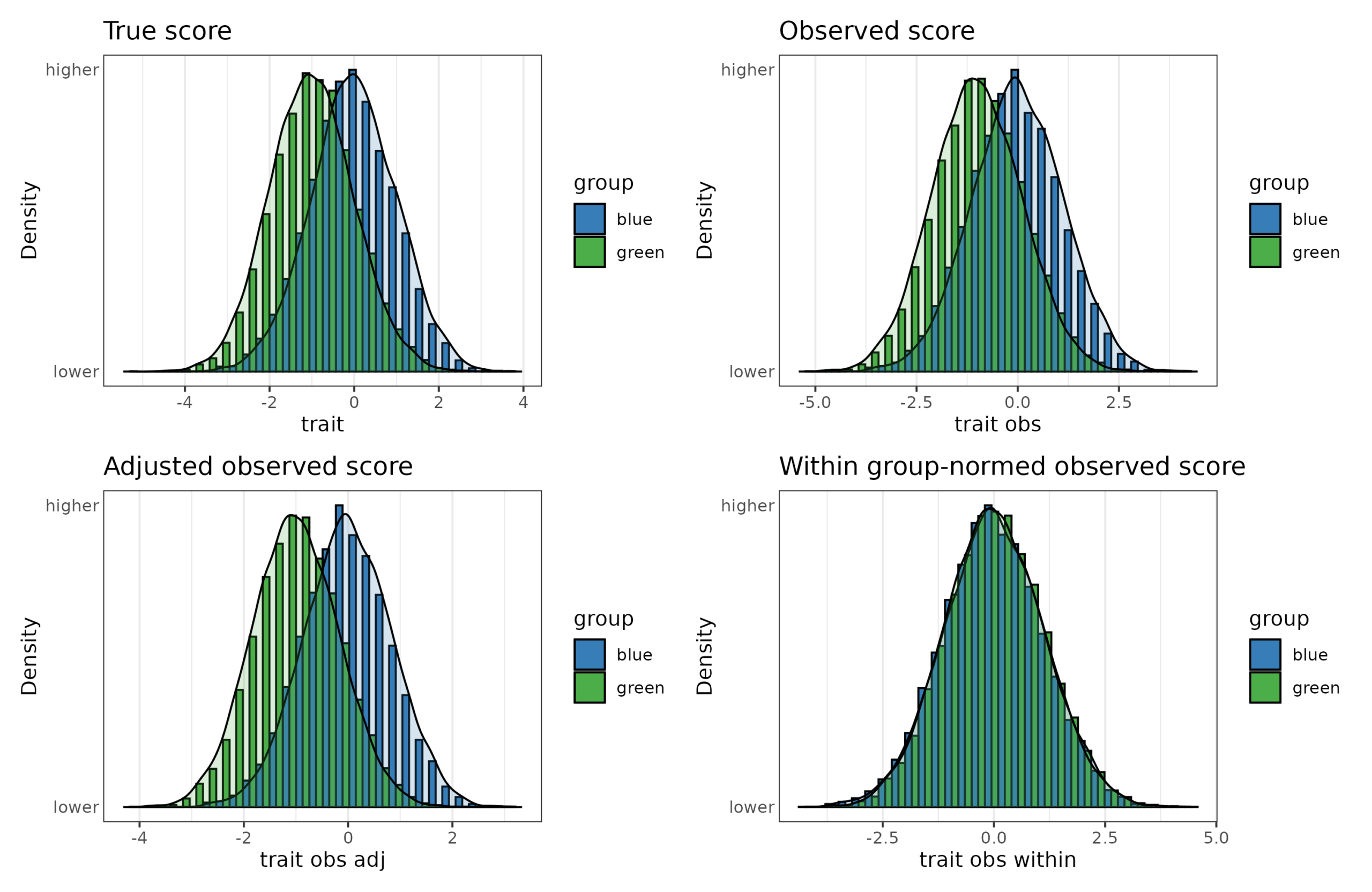
These are:

1. The true scores, that no one in reality knows.

2. The observed scores, based on the imperfect assessment.

3. Estimated true scores from the observed scores (see also): estimated_true_score = group_mean + reliability*(person_score - group_mean)

4. Within-group normed scores.

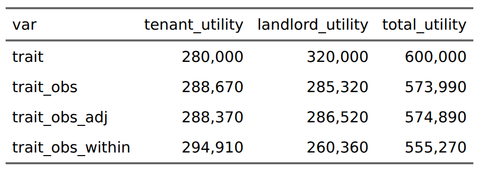
In words, (1) is reality, (2) is naive realism, (3) is skeptical realism, and (4) is strong affirmative action. One curious fact here is that (3) actually results in a larger Cohen’s d because the within group dispersion is reduced by the adjustment (d = 1.2, compared with 0.9 on observed scores). Considering the selection, we could do it using any of the 4 scores in theory, which gives these results:

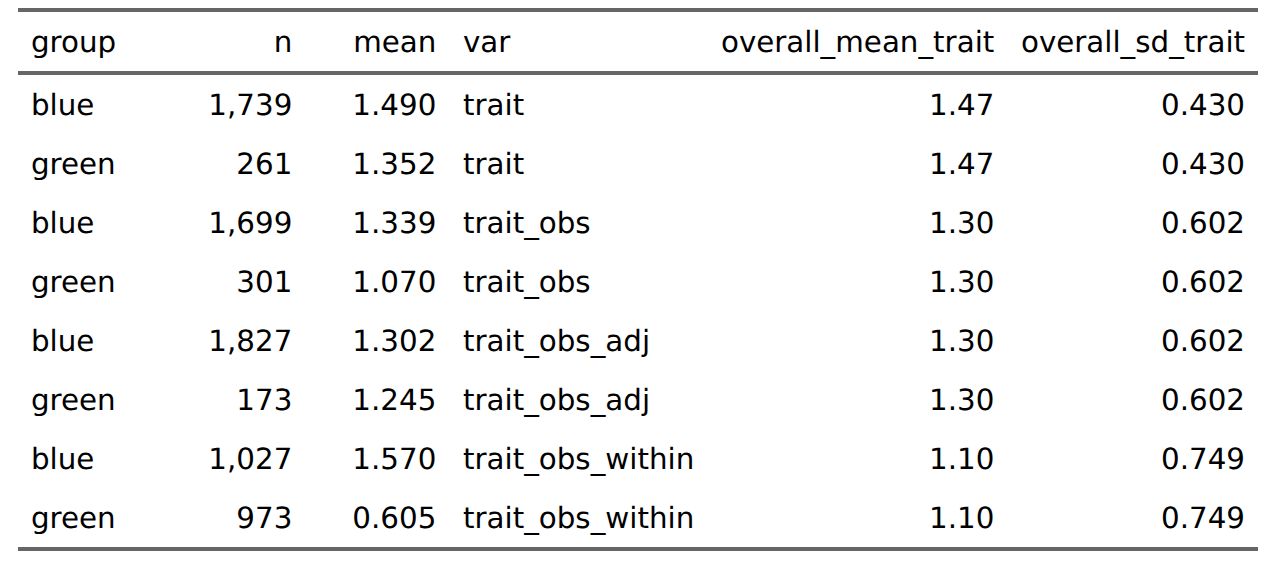
The different methods maximize different things. Selecting for the actual trait value will maximize the mean trait level of the selected persons, of course, and produce the smallest variation among the selected (sd = 0.43). Using the observed scores results in a moderate gap in trait level among those selected (1.33 vs. 1.07). Using the estimated true scores, this gap is shrunk (1.30 vs. 1.25) but fewer greens are selected (173 vs. 301). Finally, using within-group norms results in the lowest average trait level of the selected candidates (1.10 vs. 1.30) and the largest variation in trait level among candidates (sd = 0.75), as well as a sizable gap in trait level between the groups among the selected (1.57 vs. 0.61). As such, we cannot both maximize the overall trait level while minimizing the various gaps and equalizing the number of persons selected. If we say the benefit of being selected is an arbitrary unit of 1, we can calculate the benefits to the group members by the counts. In reality, there would be secondary effects downstream of the different mean trait levels in the selected group. If it represents pilots, for instance, more people will die in plane crashes if within-group norms are used, and the ability differences between green and blue pilots will be noticeable to the pilots themselves. It also recreates the problem for the next stage of selection, say, promotion, where the same group gap between the greens and blues exist (gap size post-selection is 0.97).

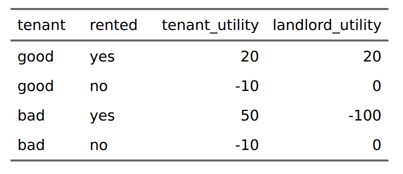
In this situation, there are no costs to anyone explicitly calculated, perhaps because everybody who applied to become a pilot but didn’t make the cut found another job afterwards. However, in many real life situations, there are costs, and they may be large. Suppose you are a landlord, and you are looking at possible tenants, some of them green, some of them blue. You don’t have the luxury of giving them some detailed assessment, you can only make a guess based on what you could glance from their online profiles and the impression they gave you on the phone. Let’s say there are secretly 2 kinds of tenants, good and bad ones. Whether a given tenant is good or bad depends again on the trait level (say, well-behavedness). Those below a score of -2 are always bad and those above are all good. As a landlord, if you pick a bad tenant, they wreck your apartment, steal your furniture, fail to pay rent, and refuse to evict. This gives you a benefit of -100 utility. A good tenant gives you 20. From the tenant’s perspective, if they are good, they also gain 20 from cooperating with you (even trade!), while a bad tenant gains 50 utils (they have fun wrecking your stuff, not paying rent, and they make money selling your furniture). Note the asymmetry here: it is easier to destroy value than create it, and the total utility of a bad tenant is -50 (50-100), or -150 if you consider the ill-gotten fails should be calculated negatively. If you don’t rent them a place to live, both good and bad tenants suffer a -10 utility from being homeless and have to live with friends and family for a while. Thus, we have the following game theory matrix:

In reality, the landlord could suffer a small cost to not renting out at all, but in this case, we consider a housing shortage. Only 80% of apartments will be rented out. The landlords will consider the information at hand and rent out accordingly. Let’s say the reliability of the impression the landlord has correlates 0.71 with the true trait level of the possible tenants, a reliability of 0.50. Now, some landlords are considering whether they should apply some of their prior knowledge about the likelihood of good and bad tenants among the blues and greens. Fortunately, both groups have a majority of people being good tenants, 97% and 84% respectively. So let’s see what happens. It get’s a bit messy, but we will be able to make sense of the numbers. First, the main utility sums:

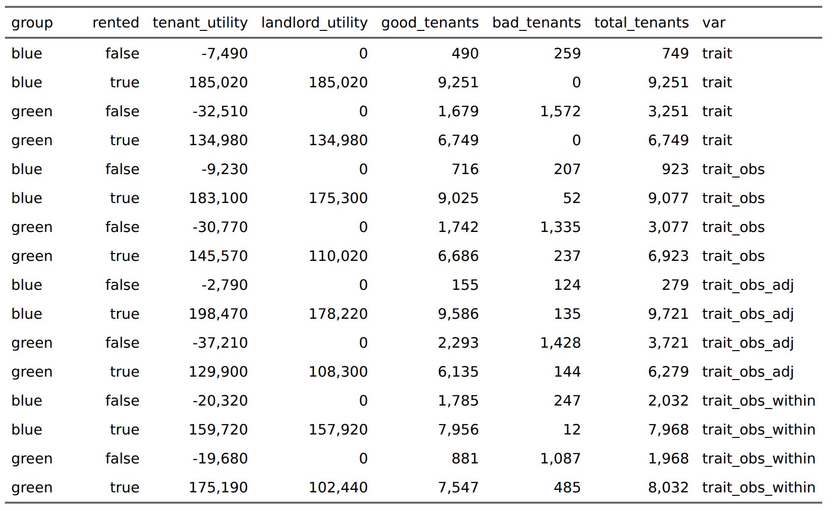
If landlords had perfect information availability, then they would never rent out to any bad tenants. This is what the first 4 rows show. Some of the people who didn’t rent an apartment would have been good tenants, but the housing shortage prevented them from getting an apartment. Next, we should look at the overall results by selection method:

Using true values, overall utility is maximized at 600k. Using whatever imperfect information the landlords could glance, total utility is 574k, the loss comes from landlords who lose out to some bad tenants they unfortunately selected. If landlords applied estimated true scores (applied regression towards the mean), utility would be marginally increased overall to 575k, at slight cost to tenants. Using within-group norms results in a substantial decrease of about 20k utility. This cost is mainly to landlords who lose 26k, and tenants gain about 6k in return. These utility includes the ones that bad tenants make because they stole stuff and refused to pay rent. Next we can consider the benefits to each group from the methods:

For the blues, the preferred situation is using the adjusted scores (196k), which are biased a bit in their favor. Otherwise, regular selection is best (174k). For the greens, however, they much prefer within-group norms (156k) to observed trait levels (115k). The tricky part here is that some of the utility gains by greens in this scenario goes to the bad tenants. We can see this by computing the sums by tenant type and renting status:

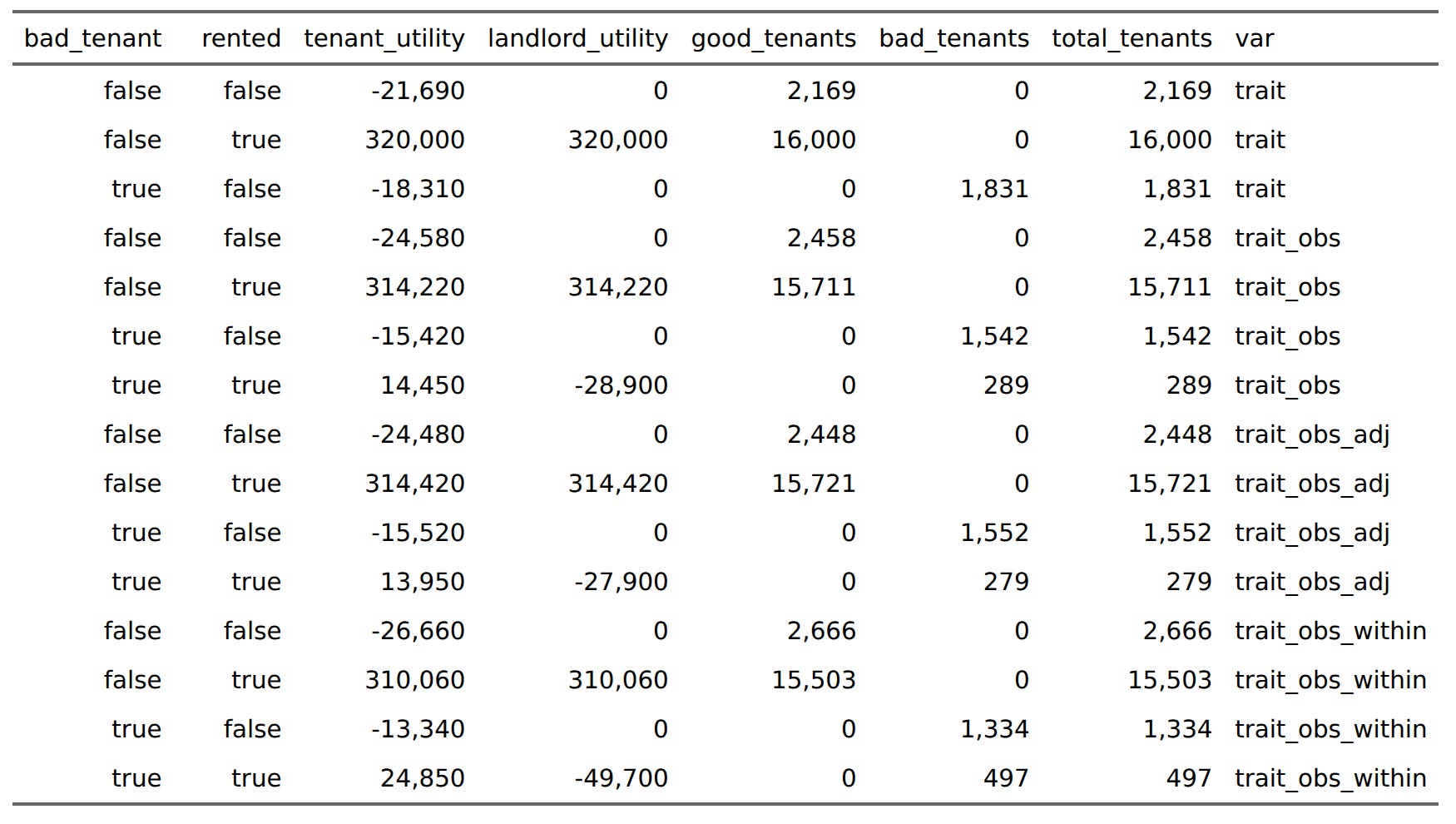
Here without splitting by color, but we can see that using within-group norms results in substantial utility gains for bad tenants, of which 497 were able to rent an apartment and trash it. If the landlords hadn’t given preference to greens, only 289 bad tenants would have gotten an apartment instead. There’s fairness angle here if we look by group and rented status:

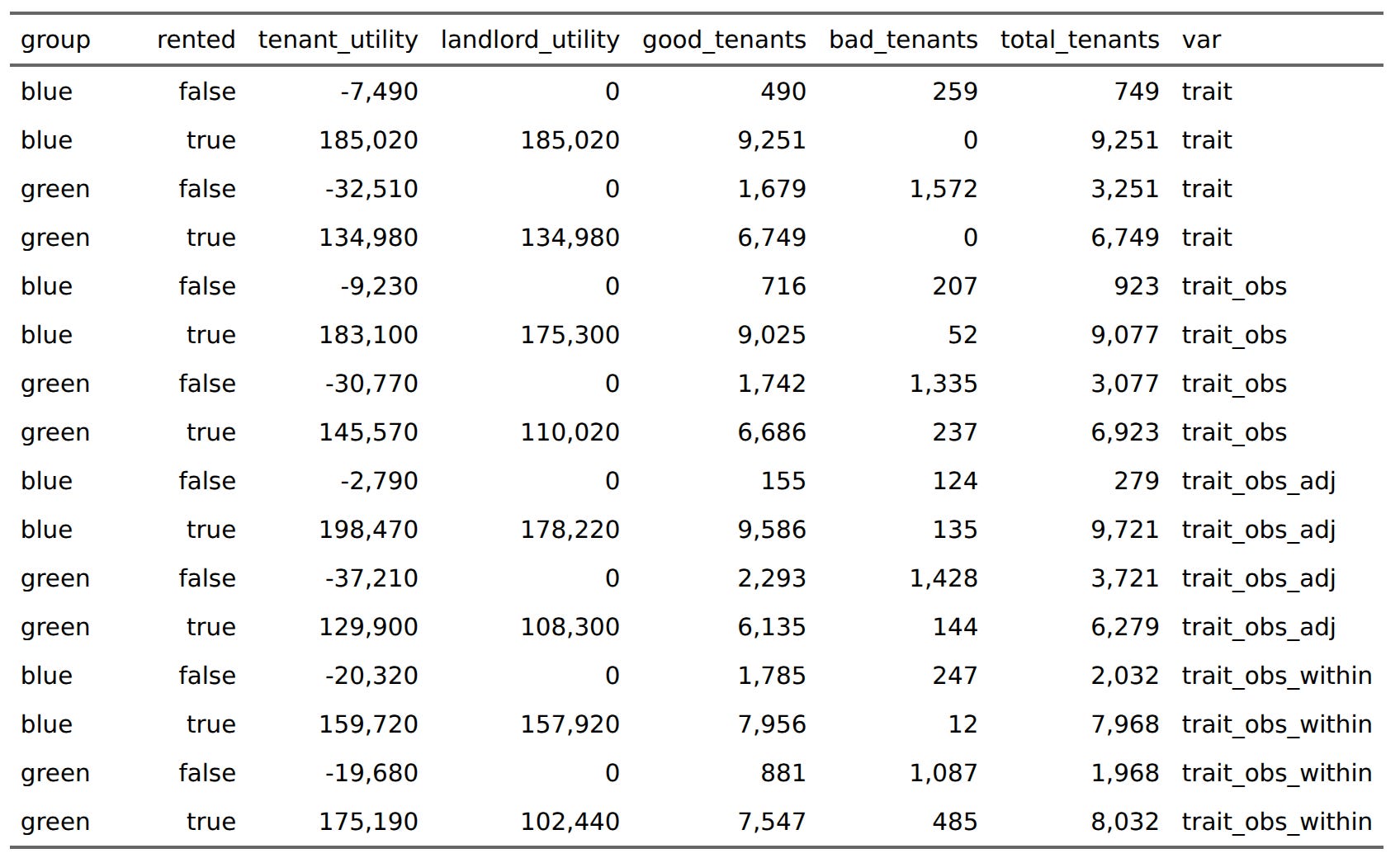
Among the greens who did not get an apartment using the observed score, a majority would have been good tenants (1700 vs. 1300). If you used the adjusted scores, the ratio changes to their detriment (2300 vs. 1400). Quite a lot of green would-have-been good tenants would be excluded using this adjustment.

One can go into more details, but I think the above illustrates my main point. When we are talking about some situation where some group or another is given the benefit of the doubt, or explicitly preference, this comes at a cost. In real life, people can fuck you over and you would be wise to reduce the risk of this happening. Any kind of affirmation action system results in a loss of total utility in cases where asymmetric costs are involved. Situations with asymmetric costs are many, they include:

• Renting, per above

• Business partners: broadly the same renting situation

• Friendships: bad friends may steal or break your stuff, beat you up, hit on your wife, or fail to pay back loans

• People on the street: may attack you

In general, whenever you are in some situation where costs are asymmetric and someone is asking you to disregard known group differences in some decision making, you would be wise to consider who is going to bear the costs of a bad decision. Applying any kind of reasonable prior to your mental score of a person is unfair to the people from the low-performing group who would have made good business partners, friends, or tenants. It’s unfair in the sense that it is not their fault that other members of that group behave poorly. However, not doing so risks substantial damage to yourself. That isn’t fair either. Why should you bear the costs of the uncertainty related to group differences? So either people from an under-performing group suffer some extra unfairness, or you suffer some extra risks. You must choose. Additionally, using any affirmative action results in bad actors accruing potentially substantial gains as well. One might consider this negative utility in the calculations. If one does, then the affirmative action total utility declines further (to 532k from 555k).

R code is here for the curious.